Principal Component Analysis

Principal Component Analysis (PCA) is a transformation technique that reduces the dimensions of datasets containing many interrelated variables while preserving as much of the variation within the data as possible. These studies were first initiated by Karl Pearson in 1901 and later developed by Hotelling in 1933. The goal is to find the optimal transformation that allows the data to be represented using fewer variables. The variables obtained after transformation are called principal components and are ordered such that the principal component with the highest variance is placed first.

Principal Component Analysis (PCA) is commonly used for the following purposes:

• Dimensionality Reduction: Reducing the number of variables in the dataset to make it more manageable.
• Elimination of Correlation Structure: Minimizing relationships among variables to obtain more independent components.
• Data Preparation for Analysis: Transforming the data into a more suitable format for other statistical analyses.

In PCA, there are two main components: the first principal component (PC1) and the second principal component (PC2).

• First Principal Component (PC1): This is the direction in which the data points exhibit the highest variance. It represents the line that best captures the shape of the projected points. The greater the variance captured by the first component, the more information from the original dataset is preserved, and no other principal component will have a higher variance.
• Second Principal Component (PC2): PC2 explains the next highest variance in the dataset and is necessarily uncorrelated with PC1; that is, PC2 is orthogonal (perpendicular) to PC1. This relationship implies that the correlation between PC1 and PC2 must be zero.

When PCA is applied, a scatter plot is typically used to illustrate the relationship between PC1 and PC2. The axes for PC1 and PC2 are shown perpendicular to each other. The first and second principal components are graphically represented below.

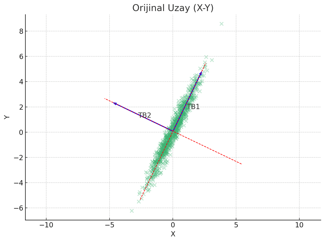
^{First and Second Principal Components (generated by artificial intelligence.)}

Let our data matrix be $M$ observation vectors, each of size $N\mathrm{x}1$, represented as $\mathbf{X}$. In matrix $\mathbf{X}$, each column represents a different variable (data type), as described below.

$\mathbf{X}=\left[\begin{array}{cccc}{x}_1^1& x_1^2& ...& x_1^M\\ x_2^1& x_2^2& ...& x_2^M\\ .& .& ...& .\\ x_N^1& x_N^2& ...& x_N^M\end{array}\right]$

Since the variables may have different units of measurement, the data are standardized. Standardization is performed by centering each variable so that its mean becomes zero. This is done by subtracting the mean of the dataset from each data point.

$\mathbf{m}=\frac{1}{M}\sum _{i=1}^n{x}^i=\left[\begin{array}{c}{m}_1\\ m_2\\ .\\ m_N\end{array}\right]$

After subtracting the means, the matrix $\tilde{\mathbf{X}}$ is obtained as follows.

$\tilde{\mathbf{X}}=\left[\begin{array}{cccc}{x}_1^1-m_1& x_1^2-m_1& ...& x_1^M-m_1\\ x_2^1-m_2& x_2^2-m_2& ...& x_2^M-m_2\\ .& .& ...& .\\ x_N^1-m_N& x_N^2-m_N& ...& x_N^M-m_N\end{array}\right]$

In the next step, the covariance matrix $\mathbf{C}$ is calculated as follows.

$\mathbf{C}=\tilde{\mathbf{X}}{\tilde{\mathbf{X}}}^T$

$\mathbf{C}=\left[\begin{array}{cccc}(x_1^1-m_1{)}^2& (x_1^2-m_1)(x_2^1-m_2)& ...& (x_M^1-m_1)(x_N^1-m_N)\\ (x_2^1-m_2)(x_1^2-m_1)& (x_2^2-m_2{)}^2& ...& (x_M^2-m_2)(x_N^2-m_N)\\ .& .& ...& .\\ ((x_N^1-m_N)(x_1^M-m_1)& (x_N^2-m_N)(x_2^M-m_2)& ...& (x_N^M-m_N{)}^2\end{array}\right]$

Variance and covariance are used to understand how variables behave within a dataset. In the covariance matrix $\mathbf{C}$ the coefficients along the diagonal represent variance values, indicating the spread of data in a single dimension around its mean. Covariance indicates how two variables change together: positive covariance means that when one variable increases, the other tends to increase as well, or both decrease; negative covariance means that when one variable increases, the other tends to decrease. The obtained covariance matrix $\mathbf{C}$ undergoes eigenvalue-eigenvector decomposition.

$C\mathbf{v}=\lambda \mathbf{v}$

Here, $\lambda$ represents the eigenvalues and $\mathbf{v}$ represents the eigenvectors. The eigenvalues are ordered from largest to smallest, and the first $P$ eigenvectors corresponding to the largest eigenvalues are selected to form the columns of the projection matrix $\mathbf{W}$.

$\mathbf{W}=\left[\begin{array}{cccc}{w}_1& w_2& ...& w_p\end{array}\right]$

Using the projection matrix $\mathbf{W}$, the dimensionality of the data is reduced from $N$ dimensions to $P$ dimensions for $i=1,2,...,M$.

${\mathbf{y}}^i={\mathbf{W}}^T{\mathbf{x}}^i$